Swin transformer is a general-purpose backbone for computer vision. This posts presents an annotated version of the Swin Transformer paper in the form of ~~line-by-line~~ code implementation. We follow the V2 implementation from Pytorch Image Models that is streamlined for educational purposes. At the end of this tutorial, we will train a model on a small dataset for butterfly classification.

Note: Please refresh this page in case latex symbols are shown properly.

The shifted window attention enables Swin Transformer to efficiently process high-resolution images with feasible computational cost while it’s pyramidal feature hierarchy can better handle the large variations of visual entities’ scales and sizes. In this guide the term patch and token are used interchangeably. We use Swin-S (Swin Small) variant with embedding/channel dimension \(C=96\), window_size = 8 and input image of size 256. This model has four stages with respective layer numbers = \({ 2, 2, 18, 2 }\) for each stage:

Here is another overview [source]:

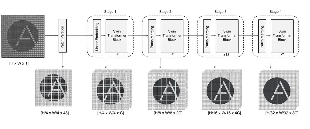
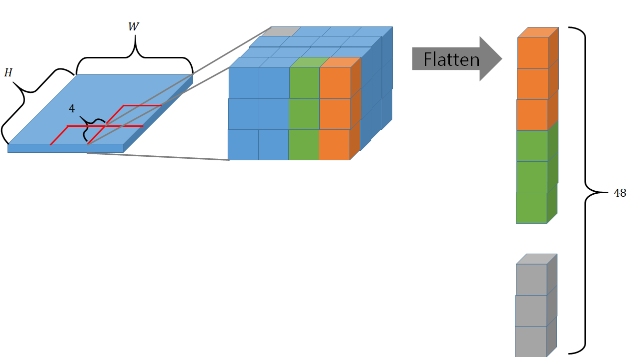
Stage 0: Patch Partition:: A linear embedding is used to flatten each patch of dimension 4x4x3=48 (4x4 RGB pixels) into a one-dimensional tensor of size 48. We have \(\frac{H}{4} \times \frac{W}{4} = \frac{256}{4} \times \frac{256}{4} = 4096\) of such patches (each with 4x4x3 = 48 dimension). Each one of these 4096 patches are used as a token for in our transformer model.

Stage 1 = Linear Embedding + STBx2: This stage consists of a linear embedding that projects the dimension of 48 of each patch into a C dimensional token. In Swin-S model we use \(C=96\). These tokens are fed into two Swin Transformer Blocks(STB). We will have a closer look at Swin Transformer Block later. At the end of this stage we get \(\frac{H}{4} \times \frac{W}{4} = (\frac{256}{4} \times \frac{256}{4} = 4096 \) patches/tokens each with dimension \(C=96\). As mentioned previously, please note that there are two of these STB’s at this stage.

Stage 2 = Patch Merging + STBx2: First there is a patch merging mechanism (discussed later) which concatenates patches obtained from the previous stage, followed by two Swin Transformer Blocks. At the end of this stage we have \(\frac{256}{8} \times \frac{256}{8} = 1024\) patches, each with dimension \(2C=2\times 96= 192\). As you can see, the number of patches are decreasing but the dimension of each on is increasing.

Stage 3 = Patch Mergin + STBx18: We have another patch merging layer, following by eighteen Swin Transfomer blocks. At the end of this stage we have \(\frac{256}{16} \times \frac{256}{16} = 256\) patches; each with dimension \(4C=4 \times 96 =384 \).

Stage 4 = Patch Mergin + STBx2: The final patch merging layer, followed by two swin transformers blocks. The output is \(\frac{256}{32} \times \frac{256}{32} = 64\) patches; each with dimensions \(8C=8 \times 96=768\).

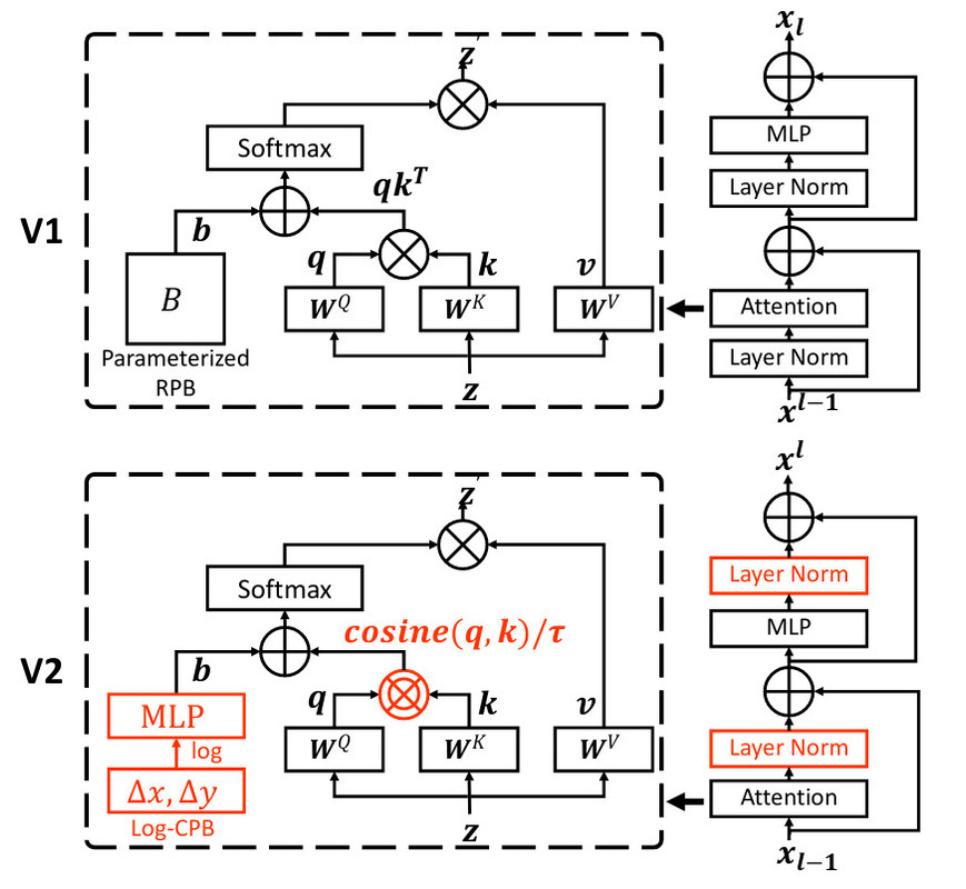
Furthermore, there are some differences between between Swin V1 and V2 architecture. Residual-post-norm replaces the previous norm configuration (Residual is the input from pre-attention). Also scaled cosine attention replaces original dot attention. Furthermore, a log-spaced continuous relative position bias approach to replace the previous parameterized approach:

Import the Libraries

First, we import the libraries we need:

Partition the Window

A window consists of collection of patches of size 4 x 4 RGB pixels. In Swin-S, each windows is of size 8x8=64 patches. First, we define window_partition function that takes an image and partition it into windows of size window_size=8x8. The number of windows num_windows is calculated automatically by this function based on the size of the window.

The next function is reverse of the function above. It takes a collection of windows and return an image:

Both the above functions are used in Swin transformer block.

Window Attention

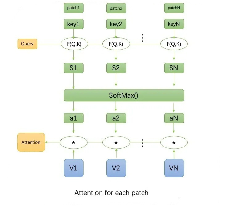
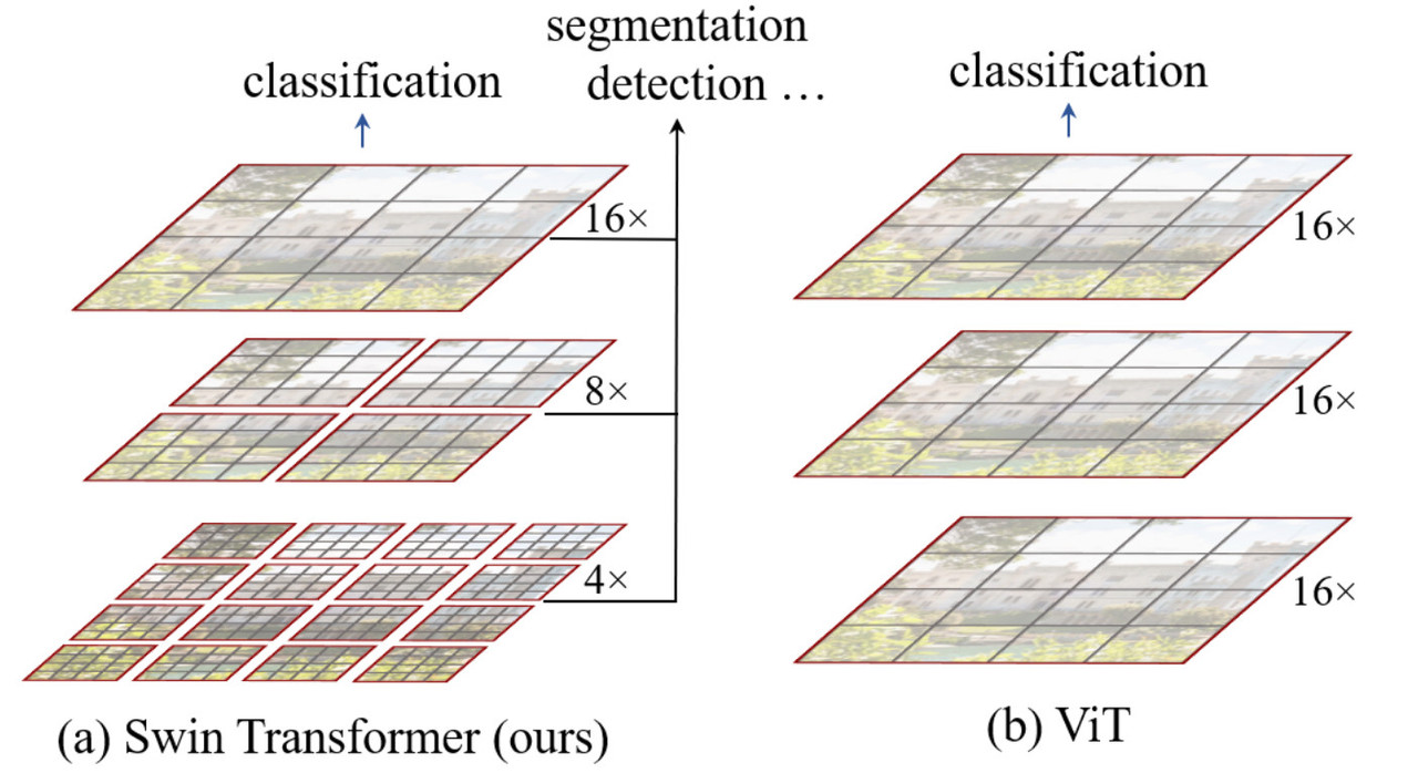
Attention is only applied locally on each window. It is NOT applied on individual pixels within a patch. In our example, the attention happens between the 8x8=64 patches in each window. The attention is local i.e. each patch attends only to the other 64 patches in its window. The query key set has 64 values only and it does not vary which is different that sliding window models. Since the number of patches in each window is fixed, the complexity becomes linear to image size, as opposed to quadratic complexity of ViT.

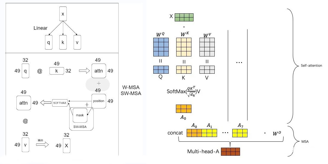
Relative Position Bias: Unlike some other architectures which use absolute position embeddings, Swin transformer attaches a so-called relative position bias \(B \in \mathbb{R}^{M^2 \times M^2} \) to each head for computing similarity. As the name suggests, it is calculated based on the relative position of a patch in a window of size M:

\[\text{Attention}(Q,K,V) = \text{SoftMax}(\dfrac{QK^T}{\sqrt{d}}+B)V \]

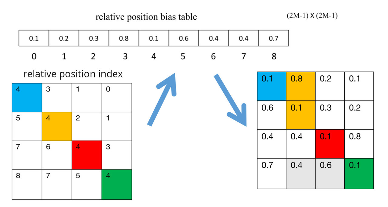
where \(Q,K,V = \mathbb{R}^{M^2 \times d}\) are the query, key, and value matrices; \(d\) is the query/key dimension, and \(M^2\) is the number of patches in a window. Since the relative position along each axis lies in the range \([-M+1, M+1]\), we parameterize a smaller-sized bias matrix \(\hat{B} \in \mathbb{R}^{(2M-1)\times(2M-1)}\) (\(2M-1\) is smaller than \(M^2\)), and values in \(B\) are taken from \(\hat{B}\).

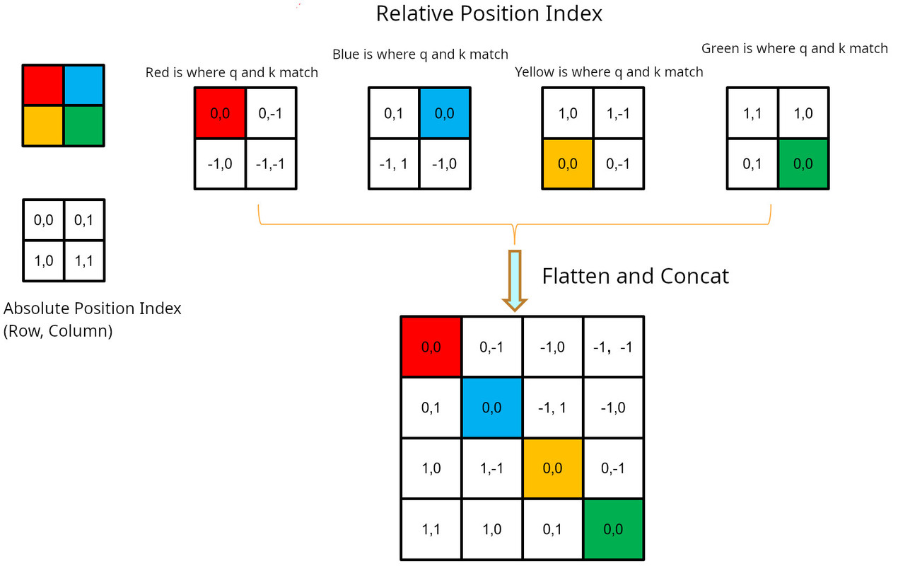
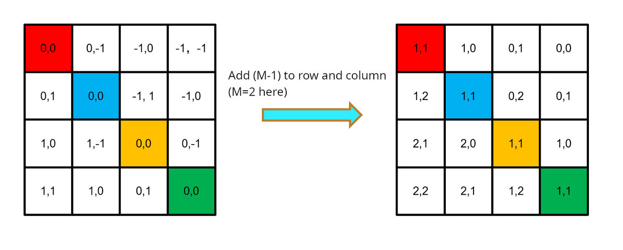
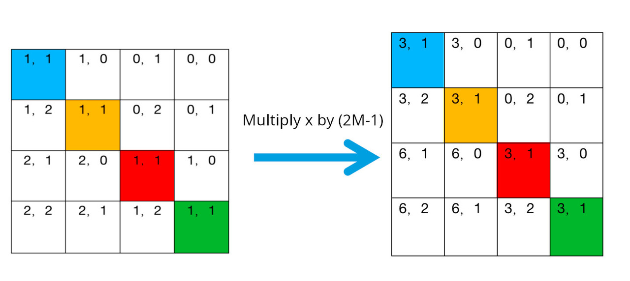
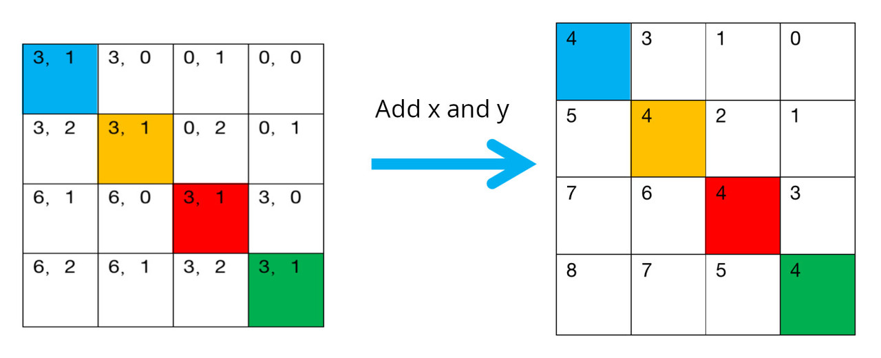
In order to calculate relative position bias, first we need to calculate relative position index. The hashing algorithm used by the authors is \( (x+M-1) * (2M-1) + (y+M-1) \) where \(x, y\) are the row and column index and M is the dimension of the window. The following dummy example shows an example with window of size 2x2:

Add M-1 to the row and column:

Multiply the first index x by 2M-1

Add x and y:

All the stops abvoe amount to section B in the code below. All these values are stored in relative_position_index.

Continuous relative position bias (Swin V2): Instead of directly optimizing the parameterized baises, the continuous position bias appraoch adopts a small meta network on the relative coordinates:

\[ B(\Delta x, \Delta y) = \mathcal{G}(\Delta x, \Delta y) \]

where \(\mathcal{G}\) (or cpb_mlp) is a small network, e.g. a 2 layer MLP with a ReLU activation in between by default. This meta network \(\mathcal{G}\) generates bias values for arbitrary relative coordinates, and thus can be naturally transferred to fine-tuning tasks with arbitrarily varying window sizes. In inference, the bias values at each relative position can be pre-computed and stored as model parameters, such that the inference is the same as the original parameterized bias approach.

Log-space coordinates (Swin V2). When transferring across largely varying window sizes, a large portion of the relative coordiante range needs to be extrapolated. To ease this issue, we propose using log-spaced coordinates instead of the original linear-spaced ones:

\[ \widehat{\Delta x} = \text{sign}(x) \cdot \log(1 + [\Delta x]) \] \[ \widehat{\Delta y} = \text{sign}(y) \cdot \log(1 + [\Delta y]) \]

where \(\Delta x, \Delta y \) and \(\widehat{\Delta x}, \widehat{\Delta y}\) are the linear-scaled and log-spaced coordinates, respectively.

By using the log-spaced coordinates, when we transfer the realtive position biases across window resolutions, the required extrapolation ratio will be much smaller than that of using the original linear-spaced coordinates. For en example of transferring from a pre-trained 8x8 window size of a fine-tuned 16x16 window size, using the original raw coordinates, the input coordinate range will be from [-7,7]x[-7,7] to [-15,15]x[-15,15]. The extrapolation ratio is \( \frac{8}{7}= 1.14x \) of the original range. Using log-spaced coordinates, the input range will be from [-2.079, 2.079]x[-2.079, 2.079] to [-2.773, 2.773]x[-2.773, 2.773]. The extrapolation ratio is 0.33x of the original image, which is about 4 times smaller extrapolation ration than the original linear-spaced coordinates.

All the above steps are shown in section A of code below and are stored in relative_coords_table.

In nutshell:

init function:
1. relative coordinates are generated and stored in ‘relative_coords_table’
2. relative position index are generated and stored in ‘relative_position_index’
3. The bias for q, k, v are initialized
forward function:
1. calculate q, k, v and use them to calculate scaled attention
2. the indices stored in ‘relative_position_index’ are used to pick values from ‘relative_position_bias_table’
3. relative position bias is added to the attention
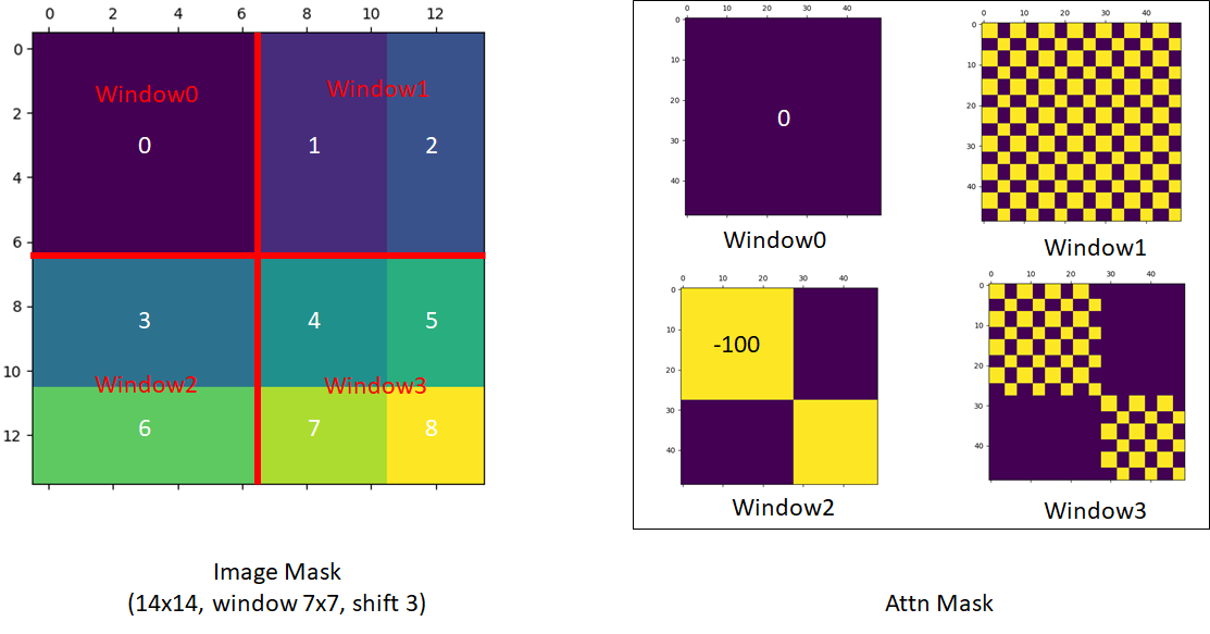
4. The mask is added to the attention. Mask has either 0 or -100 value. The patches that get -100 mask are ignored.
5. SoftMax is applied to the attention
6. v is multiplied by attention

Cyclic Shift and Reverse Cyclic Shift

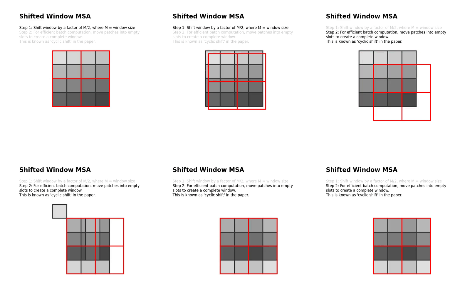
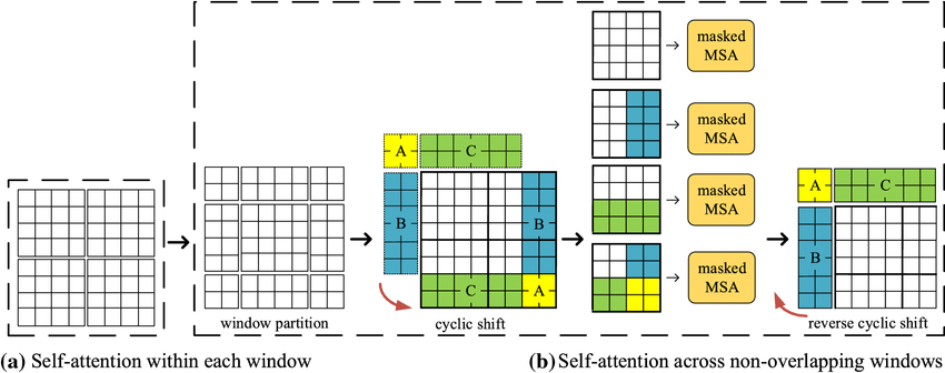
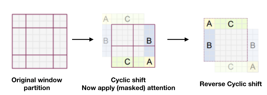
Cyclic Shift and Reverse Cyclic Shift are two important operations in Shifted Window Multi-Head Self Attention (SW-MSA). They are introduced to solve interaction between each window. In cyclic shift the window is moved by M/2 where M is the size of the window. In other words, an offset is introduced to the window in feature map. Reverse cyclic shift is the reverse operation.

Attention Mask

If Shifted Window is the essence of Swin Transformer, then Attention Mask can be regarded as the essence of shifted window. The main purpose of attention mask is to set a reasonable mask, so that Shifted Window Attention has the equivalent calculation time as Window Attention.

As mentioned before, In the Swin Transformer, in order to solve the interaction between each window, an offset/shift of size M/2 to the feature map is introduced, but after the offset is introduced, the number of windows in the source feature map increases, which increases the amount of calculation. Swin transformer author’s propose masks to address this problem.

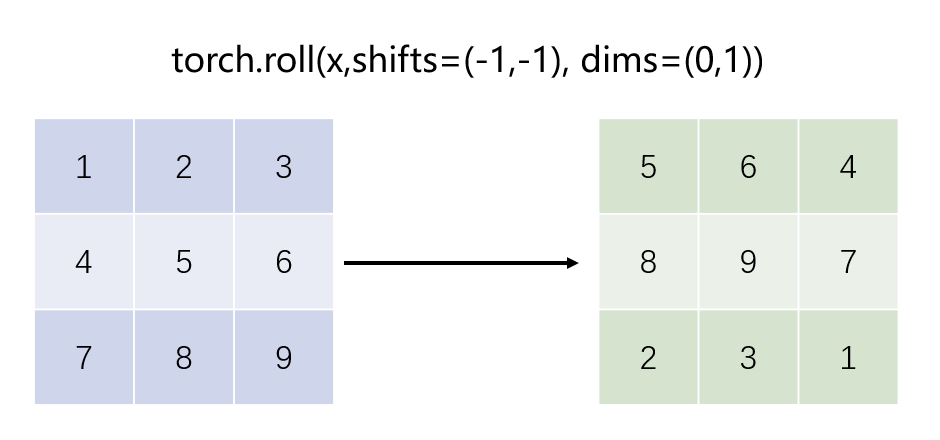
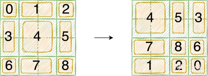
First, we index each window and do a roll operation. In the images below we show a dummy example performed on an image of 4x4 patches with window_size=2 and shift_size=1.

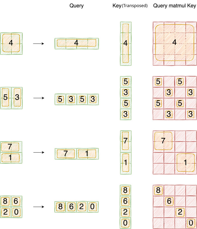
With attention mask we hope that the same index QK be calculated, and ignore the calculation results of different index QK. The final correct results are shown below: First the query is flattened and then multiplied by key.

Here is a sample code that demonstrates the attention mask mechanism source (THE code below is just for demonestration purposes. DO NOT INCLUDE IN THE PROJECT):

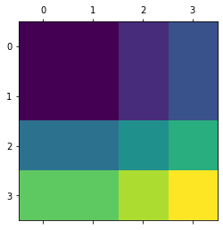
We get the following attention mask as output:

Here is the plot of the attention mask. You notice it is same as the illustration above:

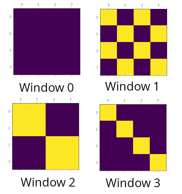
The patches that have value -100 will be ignored by softmax. Here is a more complex example with window-size=7 and shift_size=3 performed on images of 14x14 patches:

Swin Transformer Block

The Swin Transformer Block (STB) performs the following tasks:

init function:
1. Calculate window shift
2. Calculate the attention mask for the window.
attn function:
1. performs cyclic shift using .roll operation.
2. partition windows.
3. performs the shifted window multi-head attention.
4. perform reverse cyclic shift.

Also note that first the embedding dim of 96, 192, 2 * (previous step’s dimension). The output resolutions is decreasing with dimensions H/16 * W/16 and H/32 * W/32, so on while the embedding size increases by 2 each time.

Patch Merging (Downsampling)

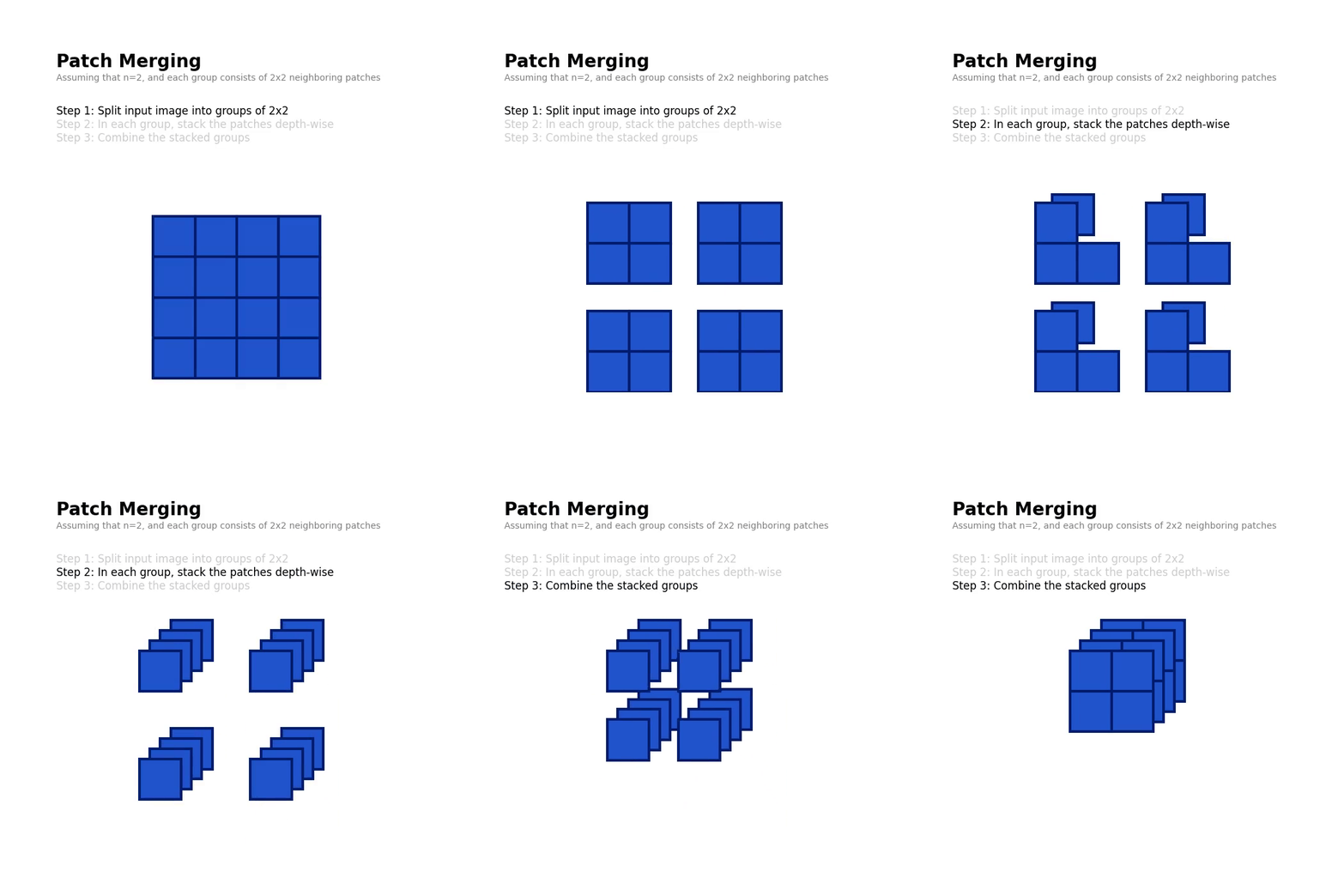
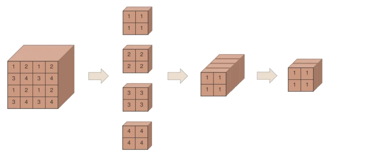
Patch Merging groups each n x n neighboring patches and concatenates them depth-wise. This effectively downsamples the input by a factor of n, transforming the input from a shape of H x W x C to (H/n) x (W/n) x (n^2 * C), where H, W and C refers to the height, width and channel depth respectively.

The purpose of patch merging is to perform downsampling before the start of each stage in order to: 1) reduce the input resolution 2) adjust the number of channels to form a hierarchical design 3) and also save a certain amount of computation. This is similar to striding=2 in CNN, the convolution/pooling layer is used before each stage to reduce the resolution.

Here is another figure [source]:

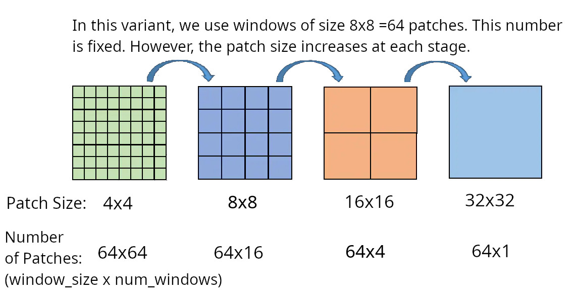
Note that while the size of the windows is fixed (8x8), the size of the patches increases while the number (not size) of the windows decreases:

Patch merging reduces the number of tokens (patches) at the cost of increased dimension. The first patch merging layer concatenates the features of each group of 2 × 2 neighboring patches, and applies a linear layer on the 4C-dimensional concatenated features. This reduces the number of tokens by a multiple of 2 × 2 = 4 (2× downsampling of resolution), and the output dimension is set to 2C.

The image below shows patch merging in Swin architecture vs ViT architecture. The Swin transformer does the calculation of self-attention in each window and obtains an updated window. It then merges the windows through the operation of patch merging, and then continues to do self-attention calculation.

Each downsampling is doubled, so elements are selected at intervals of 2 in both row and column directions . Then spliced together as a whole tensor, and finally expanded. At this time, the channel dimension will become 4 times the original size (because H and W are each reduced by 2 times), and then adjust the channel dimension to twice the original size through a fully connected layer. Below is a schematic diagram (input tensors N=1, H=W=8, C=1, excluding the final fully connected layer adjustment)

Basic Layer

We have four basic layers or stages. At each stage (or basic layer) we create 2, 2, 18, and 2 Swin Transformer Blocks and perform patch merging.

Swin Transformer V2

Here is where all the pieces come together. First we split the input into non-overlapping patches using PatchEmbed function of timm library. This amount to stage 0. Then we create the four stages (or basic layers) of swin transformer architecture. The forward function comprises two functions: forward_features and forward_head. First function does the feature training while the latter computes the head which is a linear transformation from num_features to num_classes (there are 1000 classes in our butterfly example). num_features is calculated by the formula int(embed_dim * 2 ** (self.num_layers - 1)) which is calculated to int(86 * 2 ** (4 -1)) = 768.

Create the Model

We optimize the pretrained weights on Imagenet22K for our butterfly dataset. This greatly reduce the training time while achiving a satisfactory 92% accuracy on this relatively small dataset. To create our model, First we got to make sure that buffers that are not persistent are ignored.

Butterfly Classification

First download the dataset from here and extract it. Our dataset has 9285 train images, 375 test images, and 375 validation images. Each JPEG image has 224 X 224 X 3 dimension. We then proceed to prepare the dataset: (make sure you edit dataset_path to reflect your local dataset path):

Then we make our model and we train it. The entire training time on a Nvidia 3080TI is around 4 minutes:

Let’s see he performance of our model on the test dataset:

Here is the output: